Flying the T-6

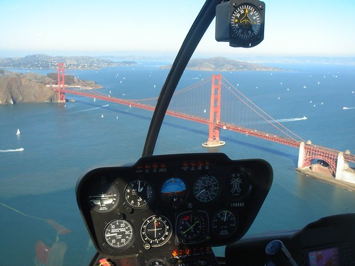
One of the many good things about Attitude Aviation is the variety of exotic aircraft that you can fly there. You can fly a Pitts and even, with enough time, patience and money, get to the point where they'll let you solo it or take friends for hair-raising aerobatic rides. They also have a Waco, which is a huge, lumbering - but aerobatic - biplane of pre-WW2 design, and a Marchetti, which is a nice touring airplane that just happens also to be fully aerobatic, including inverted. Not to mention the L-39 which allows you, at eye-watering expense, to fly a jet.

And recently, they finally got their T-6 (also known as a Texan, or in the UK a Harvard) back on the line. This is another WW2 design, classified as an "advanced trainer". In those days, a 19-year old would start flying a Stearman, solo after a handful of hours, and after getting to barely double figures would find himself behind the stick of a 550 HP monster, the size of a combat fighter. A few tens of hours in that and he'd be in a Spitfire, Hurricane or P-51, in combat for real. And maybe he'd come back, too... or maybe not.

Attitude originally had the T-6 on the line a few years ago. I flew it a couple of times, partly to prepare myself for flying the P-51 - but that's another story. Soon afterwards it had a landing mishap. The saga of the repair work and repaint that followed makes for a very long story - but finally, two years later, she showed up again at Livermore airport. I felt I needed to do something to celebrate getting my commercial pilot's license, so the timing was perfect.

The first thing about the T-6 - compared to the normal small planes we fly - is that it is seriously big. The low-mounted wing is at chest height, and the canopy stands about ten feet above the ground. Getting into it involves first clambering up on to the wing, then hoisting yourself into the cockpit, standing initially on the seat before you carefully lower yourself into place. There are two beams for your feet, with rudder pedals at the ends, and underneath that a huge void. Whatever you do, don't drop something in there!  All the controls are massive. It feels truly indestructible. After all, they were made to take tremendous abuse from very inexperienced pilots.

It's also been said that they were specifically designed to embody every known defect of all the combat aircraft of the time. So no matter what you eventually found yourself flying, it would seem tame compared to the T-6. One thing to do the first time you fly a new type - especially if it's as different as this - is to get familiar with all the controls. This means sitting in the cockpit, manual in hand, making sure you know where everything is and what everything does. Maybe you even move some of the controls. But whatever you do, don't move the landing gear control. Because this aircraft has no protection against that - move it to the "retracted" position while on the ground, and it will obligingly tuck the wheels up under itself, doing a lot of expensive damage in the process.

Finally, you feel ready to go flying (with an instructor - this is not a plane that Attitude will let you solo). The first thing to do is start the engine. It's not like a car, this is not a trivial matter. First of all, the prop must be manually turned through a couple of revolutions. Big radial engines like this are notorious for getting puddles of oil in the lower cylinders. Oil being incompressible, if the engine starts like this, the cylinder will be wrecked. This would be highly embarrassing, as well as expensive.

That done, you can climb back into the cockpit, and do battle with one of the most frustrating pieces of equipment on the aircraft. Like most piston engines, this one needs priming - using a manual pump to squirt raw gasoline into the inlet manifold. But the pump is incredibly stiff, and once you're strapped in it's at arms-length. I confess to having been completely unable to unlock the pump, needing someone else to climb up and do it for me. Though not expensive, this is definitely embarrassing - a bit like not being able to release the old-fashioned parking brake on your first driving lesson.

Finally, four shots of primer, and the primer has been closed and locked again. The starter is, uniquely, operated by a pedal between the rudder pedals. As soon as the engine fires, you must get back smartish onto the pedals, to be sure the brakes are fully applied. At the same time, you have to get the engine actually running. Radial engines start one cylinder at a time, or so it seems. The first kick must be carefully nurtured, the throttle advanced very slowly, as (hopefully) another cylinder starts to fire, and another, to the accompaniment of loud bangs and the occasional flame from the exhaust. Watching someone else start a radial engine (and listening to it!) is a delightful experience. Doing it yourself is fraught, with the knowledge that if you fail you'll have to start over, including the dreaded primer.

Finally the engine is running smoothly, all cylinders firing. Now it's time to taxi. As you release the brakes and start to move, you realise just how huge this thing is. Luckily the brakes are conventional - not heel brakes, or the strange composite arrangement with a bicycle brake lever on the stick like on the L-39. But it can't be too easy. In a taildragger you want to keep the stick fully back all the time when on the ground (let's ignore quartering tailwinds for now). That locks the tailwheel within a narrow range of motion. So if you want to make a tight turn, for example to reverse direction in the runup area, you must release the tailwheel lock by moving the stick forward. But for takeoff, it's vital to have it locked. And of course sometimes  it doesn't just lock itself - you have to wiggle the aircraft to and fro, until everything is right.

So, you've been through the (long) pre-flight checklist, got the oil nice and warm, taxied into position, and you're ready to take off. This is the frightening bit - first because you have no idea how it will behave when you apply power, and second because once you've taken off, you will, sooner or later, have to land again. (A very experienced Pitts pilot once told me that it took him several hundred flights before his first thought on becoming airborne stopped being, "Oh, sh*t, now I have to land it!").

The T-6 is actually fairly docile as it rolls down the runway. It doesn't have any vicious habits. It does take some heavy footwork to keep it rolling straight, especially as you bring the nose up. And, unlike the Pitts, it rolls a long way - although it has 550 HP, it weighs a lot too. Finally it reaches rotation speed, and with a pull on the stick you're airborne.

We flew over to our usual aerobatic practise area, which gave some time to get a feel for the aircraft. The stick is quite heavy but easy to get used to. It doesn't have a lot of adverse yaw (unlike the Citabria, for example) so only modest rudder inputs are required. And it makes that wonderful radial noise as you putter along at a modest power setting and 130 mph or so. You just know that everywhere you go, people are looking up and thinking, "What's that?"

We did a few of the usual exercises with a new type, starting with turns and then steep turns. They're easy to fly, the forces, while heavy, are consistent and well balanced. Then we went on to simple aerobatics - loops and rolls. These, too, went easily enough. It takes a lot of force on the rudder to keep a roll straight, and because the roll rate is not very high, the loop finishes with the nose pointing distinctly downwards. Loops go nicely enough, diving for 180 mph then pulling round at 3.5G or so.

Once in flight, the T-6 flies fairly unremarkably. You forget its size, since it doesn't really matter up there. The panel is typical of its era - there's no six-pack, just instruments and switches dotted about at random. The landing light switches, for example, are on the left of the main panel - while all other lights are on their own panel on the right side of the cockpit. (I confess that I didn't find them in flight when I wanted them). The fuel gauges are even worse. They're purely mechanical, with sight gauges down in the void under the floor on either side of the cockpit. Before strapping in I did manage to locate them, but I found reading them in flight to be impossible. The gear lock confirmation is similar - you have to look through two tiny windows in the upper surface of the wing, to see the yellow lock pins. I said I could see them, and at the time I convinced myself that I did, but to be honest it's pretty questionable.

We did a couple of stalls, which were also unremarkable. Then it was time to go and land - with a wonderful view of Mount Diablo in the setting sun. I had an unpleasant experience landing a much smaller vintage taildragger a couple of years ago, so I get a bit apprehensive at this stage. With the T-6, the plan was to wheel-land it. Smaller taildraggers are normally landed on all three wheels at (much) the same time, but with bigger ones it's common to land with the fuselage level, just on the main gear. This means that the wings are still flying and will happily bounce back into the air if the tail drops, increasing the angle of attack. So you have to "stick" the airplane by pushing the stick forward at touchdown. Timing and finesse are everything - too late, and you bounce. Too early, and you thunk painfully hard into the runway - and then bounce. Too much, and you can ding the prop as the nose drops towards the runway.

As it turns out, the T-6 is a pleasure to land. Maintaining a steady 95 mph on final, just gently lowering the main gear onto runway then pushing the stick forward give a gentle touchdown. It's much easier than a wheel-landing in a Citabria!

The flaps on the T-6 are odd in a couple of ways. First, they're "split flaps" - all of the action happens under the trailing edges. From the cockpit the wings look solid, and when you move the flap handle, nothing visibly moves. All the action is underneath. In consequence, it's easy to forget to retract them after landing. And if you forget them until after shutdown, you have a problem. They are operated by an engine-driven hydraulic system, and once the engine has stopped, the only way to retract them is with a manual pump somewhere in the bowels of the aircraft. Guess how I know.

We did a couple of touch-and-goes, which went rather well, then we returned to base. My one real landing didn't go so well - I dropped in hard enough to elicit comment, rather than the smooth touchdown I'd managed earlier. And I'm afraid to say I was a bit heavy-footed on the rudder. I think I've got so used to the Pitts, which is very controllable and reactive on the rollout and will forgive a surprising amount of clumsiness, that the much more leisurely response of the T-6 caught me unprepared.

So, finally, it was back to Attitude, and engine shutdown. The sun was just setting as we landed, so the usual post-flight photo opportunity gave some nice sunset-type shots.

And some time, I really will have to spend some time just getting comfortable with landings. Apart from that the T-6 is a pussy cat, albeit a very big, heavy (and expensive) one.

Solar Power - so far, a mixed success

One of the unexpected benefits of losing my job was that my wife, who had taken over paying the household bills, took a close look at the power bills and had conniptions. She decided right there to get a solar power system installed.

This was quite an undertaking - the roof was getting old so we decided to have that redone at the same time, which in turn involved overhauling the solar heating panels for the pool which were there. The couple of weeks before Christmas were extremely noisy and dirty as big, strong men jumped up and down on the roof.

Now, the installation is complete - well, we've paid all the bills anyway. PG&E came by yesterday and installed the new meter, so now we can sell them electricity, That's good. But sadly, it isn't actually working completely, and it's not clear whether the problems can be fixed. That's not so good.

The system consists of 26 separate panels mounted at a slight angle on the roof, facing slightly east of south. Why they didn't make them face true south, I have no idea. We went for the highest-tech system on offer, using high grade panels from SunPower, each with its own inverter. This allows each panel to function separately and optimise its use of the available light, rather than wiring them in series so the output is always set by the weakest. This also allows us to get accurate real-time reporting of the power generation. At least, it should.

Our first problem is some trees on a neighboring property. In the winter (i.e. now), they start to shade the panels from about 11.30. From the pretty graphs the system produces, I can see that we're losing about a third of the production due to those trees. Generally I like trees, and I don't particularly want them cut down, even if the neighbor would agree. What is really annoying, though, is that if the panels had been placed differently on the roof, the shading would not have been as bad. This is something that the survey should have caught, and didn't. Once the sun is higher in the sky, I guess from some time in March, this won't be a problem. But still, it is probably going to lose us 10% or so of the total annual production.

The second problem is with the "fancy technology" part of the system - specifically, the Envoy box that monitors the panels and sends the data off to a company called Enphase. This is a Kleenex-box sized gadget, which communicates with the panels over the power line. This makes perfect sense rather than running a second set of cables. Or at least, it would make sense if it worked.

Initially this box was in my office, next to the router which it also needs to be connected to - by a cable, since for some reason they didn't use WiFi. That didn't work because the data-over-power couldn't get a good enough signal. So they moved it to the garage, close to the breaker box. That meant installing a second, completely separate, powerline bridge to carry the data.

I've always been suspicious about data-over-power. The idea of mixing all those tiny, sensitive little data bits with all the noise, inductive loads and general mess of electric power just doesn't seem like it should work - try connecting an oscilloscope to your power line and you'll see what I mean. I suppose I should feel reassured that it doesn't work. It's just that I'd rather it did.

Two of the panels simply don't show up on the Envoy. When I queried this, it turns out that the data signal to the panels isn't strong enough. "You'll have to move it to an outlet closer to the panel," the installer said. Well, but there isn't one. I tried anyway just moving it to another outlet. (The thing takes up two outlets, incidentally, and must not use any kind of an adapter or extension cord). But this time, the powerline bridge didn't work. And given that, there was no way to find out whether the communication to the panels was any better or not.

For now, we're stuck. The controller can only see 25 out of the 26 panels which are installed, at great expense, on the roof. It isn't clear to me whether the 26th panel is actually able to generate any power under these circumstances - since it's the one that receives the worst shade, maybe it doesn't matter much!

Even with the system as it is, there's a certain satisfaction to paying less to PG&E each month. But it would be even better if it worked properly, considering what we paid for it.

Instrument Flying by Helicopter

My latest flying training project is to work towards my commercial helicopter license (CPL-H). Having, finally, got my airplane commercial a couple of months ago, it seems like an obvious thing to do. So my plan over the next year or so is to gradually "tick all the boxes" for the experience requirements for the CPL-H, as described in FAR 61.129(c).

One of these is to get 5 hours of "actual or simulated instrument flying". Since our Robinson 44 is not allowed to fly in actual conditions (i.e. in clouds), this means flying "under the hood", using a gadget which restricts the pilot's view to just the instruments. This is how most instrument training and currency is done, even in airplanes, since you can't really count on clouds to be there when you need them, especially in our part of the world. Yesterday I completed my second helicopter flight under the hood, amounting to a magnificent total of 3.4 hours so far.

In a plane, with its high glareshield, there are lots of effective ways to limit the pilot's view. I use something called "Foggles" which are like industrial eye protection goggles with most of the lens covered in a translucent film. Only the bottom part, corresponding roughly to the reading part of bifocal glasses, is left clear. As long as the pilot isn't actually trying to cheat, these do the job very well. In fact, it's surprisingly easy not to cheat, assuming your goal is to be trained rather than just to pass a checkride. (In the latter case, it isn't really worth trying to cheat because the examiner will notice immediately). I remember one flight, on my own in actual cloudy conditions, where I popped out of the cloud and it took me a while even to realise that I didn't have to rely on instruments.

In the helicopter, it's harder to do an adequate job of restricting vision, because the visibility is so much better. The only thing that works - and then not very well - is the decidedly steampunk Francis hood, looking like something a submarine commander should be wearing. Even so it's impossible not to see ground through the lower part of the canopy - you just have to try not to notice it.

Flying the helicopter under the hood is much harder than a plane. For a start, you can't take your hands off the controls. A plane will cheerfully fly for tens of seconds, hands off. You sometimes see a plane referred to as a good "instrument platform", meaning that it is naturally stable. My own Cessna TR182 falls into this category. The heli, on the other hand, always requires a hand on the cyclic (the up/down/sideways control corresponding to the stick or yoke in a plane). Normally it's your right hand, but you can switch hands if you need to, for example to twiddle the Garmin 430 in the usual R44 instalation. Even that is tricky - it's difficult to fly as smoothly with the "wrong" hand (I guess left-handed helicopter pilots may find the opposite, but probably not - it's all a question of habit). And you have to be constantly prepared to get a hand on the collective really fast if the engine stops, to enter autorotation in the couple of seconds you have before the aircraft simply drops out of the sky.

Flying, and especially instrument flying, involves a lot of fiddling round with bits of paper - charts, approach plates and so on. It is very difficult to refold a flimsy IFR en-route chart with just one hand. For this reason, IFR-approved helicopters have either a crew of two, or an autopilot (or both of course). But helicopter autopilots are eye-wateringly expensive - little change out of $100,000 - and anyway not available for training aircraft like the R44. So, even during an instrument checkride, the instructor (or examiner) can be used as an "autopilot".

I've done a lot of airplane instrument flying, both under the hood and in real clouds. Much of it has been partial panel, i.e. without a functioning attitude indicator, which generally mysteriously "fails" at the very start of my instrument currency flights. So much so, that I've got used to flying without using it very much - the turn coordinator and the altimeter work just as well. That absolutely does not work in the heli, at least not at first. It is so much more sensitive that the AI absolutely has to be the primary reference all the time, just like it says in the IFR manuals. It took me a little while at the start of my first flight under the hood to realise this. Once I did, my flying became a lot more stable. In an airplane, quite a casual instrument scan works fine. But in the heli you really have to be moving very quickly between all the instruments. It takes only a small distraction to suddenly find yourself in a 30 degree bank or a couple of hundred feet off altitude. This is especially a problem when tuning radios or fiddling with the GPS - you have to scan back and forth between the AI and whatever you're twiddling, making the latter just an extra part of the scan. It's hard.

Once cruise flight is mastered, or at least under control, the next thing to tackle is approaches and holds. In principle an approach is just flying, but there's a lot more to keep track of - altitudes and headings change, and there's radio work too. A general problem with instrument flying is what happens when you get overloaded. You can go very quickly from feeling comfortable to being on the edge of complete panic, not because anything has gone badly wrong but just because there is so much to keep track of. Then small things start to go wrong - altitude and heading deviations, maybe a bit of an extreme attitude - and that piles on the workload too. It takes self-discipline to take a few deep breaths and get back to focusing on basic flying, get straight and level again, go around if you have to. For some reason the hood adds to stress too - flying in actual clouds, without the hood, seems less daunting. This may be just a very basic animal reaction to not having complete vision.

The handful of approaches I've flown have worked out pretty well, all things considered. My first helicopter ILS was the long, long descent into Moffett (KNUQ). Although it's charted as a series of step-down fixes, in practice you can fly the whole thing down the glideslope, all the way from HOOKS - 20 miles out and 5500 feet above the field. It's probably the longest ILS descent in the world, 15 minutes or so of following the needles. Fixed-wing, I flew it once with everything covered up except the VOR head - everything done by making tiny corrective inputs as the needles start to drift. It's a great exercise, but I'm certainly not ready to do it in the heli just yet!

What next? I only need one more flight like this to "tick the box" for my CPL-H. A helicopter instrument rating is pretty useless, since it's unlikely that I'll ever fly one that's equipped for IFR. But there again, it might be fun to do after the CPL-H - amazingly, it only requires another 10 hours of hood time to meet the legal requirements.

Algorithm Design: Efficient LDPC Encoding (Part 4: Optimization)

In Part 3, I described the implementation of the algorithms for reducing an LDPC code to an encodable form. At that point, all the algorithms were the most efficient possible. The only remaining performance gains would come from improving the code. This is rarely worth spending too much time on, but in this case the overall performance is completely dominated by two inner loops. One iterates through a sparse representation of a row, adding it to a dense row. The other iterates along the elements of the dense representation, adding them. Halving the time spent in both of these loops - just a few instructions each - will halve the execution time of the whole algorithm. So it's worth taking a close look.

Let's start with the add-sparse-to-dense loop. The original code used conventional STL iterators to scan through the elements of the sparse row, then for each element, converted it to the offset-and-mask combination for the particular bit number, and applied it using an xor operation. It's the obvious way. But each sparse row is added to a dense row tens of thousands of times, so it's worth considering whether any part of this operation can be amortized.

The final solution was to pre-calculate a vector containing the offset-and-mask for each entry. The latter was actually represented as a class, called "bitref". In the source code, this results in a vector<bitref>, which is iterated through in the usual way. The compiler is nevertheless clever enough to inline all this and reduce the inner loop to just four machine instructions: two to extract the offset and mask, one to perform the xor operation, and one to advance to the next entry. Not bad. Performance was improved substantially, reducing the time for phase 2 of the algorithm by a factor of about three.

There remains the overhead of the loop. Given the tiny size of the content, the two instructions of loop overhead, and their impact on pipelining, are worth worrying about. In assembler, the obvious way to unroll the loop would be to lay out sequential instructions corresponding to its maximum size, then jump into these at the appropriate point corresponding to the loop size (i.e. the number of entries in the vector). This is difficult to do in C++ though.

In the end I came up with something similar, but with a distinct unrolled loop for each possible size. This was done as my first tiny adventure in C++ template metaprogramming, and is described here. The compiler is smart enough to translate the switch statement based on vector size into an indexed jump, which then executes the entire loop in a straight line. That gave me about another 5% improvement.

Having got the inner loop as tight as possible, it was time to think about the next layer of the loop. Gcc does a good job of inlining functions when it's the right thing to do, but examination of the assembler output (-S option) showed that it was not inlining a couple of critical functions here. I played around with the compiler parameters that control inlining for a while and things got a little better, but I could just not convince it to inline one critical function. Of course the "nuclear option" of making it a macro always exists, but I really wanted to avoid that. I tried the "flatten" function attribute for the outer loop, which tells the compiler to inline absolutely everything, but after the compiler had run for half an hour or so I stopped it. I think it got put off by all the calls to boost::format that I use in my debug log macros.

Eventually, I found a minor rearrangement of functions that got everything inlined. That gave me another 5% or so performance improvement.

That dealt with the inner loop of phase 2, adding sparse rows to dense rows. In phase 3, the inner loop is adding dense rows to dense rows. Unrolling this loop was easier since it is always over the whole length of a dense row - over 64K bits, or 2K operations. There's nothing to be gained by completely unrolling such a loop. Instead I changed the code to do it in "gulps" of 16 entries at a time, then used a normal loop to deal with the remainder at the end. I also rearranged things here so that the call to the inner loop was fully inlined.

And that is about as far as things can be taken. The original C++ code took about 400 seconds for a column-weight 3, 32K data bit code. The final code takes under 7 seconds. I never ran a column-weight 5 code to completion with the original code - it would certainly have taken thousands of seconds, maybe much more. But now, it runs in about 45 seconds.

Of course there's a price to pay for all this. One of the first principles of writing maintainable systems is never to keep the same information in more than one way. This code violates that all over the place - for example, the sparse and dense representations of rows. But without this kind of approach, the code would be unusable anyway, so its maintainability wouldn't matter much. It has certainly been one of the most interesting bits of programming I've undertaken in a long timer.

Algorithm Design: Efficient LDPC Encoding (Part 3: Implementation)

In Part 2 I described the algorithms that need to be implemented in order to transform the base matrix of an LDPC code into a reduced form that can be used by a practical encoder. As I mentioned in Part 1, we originally built a very straightforward Python implementation, where the matrix was represented literally as a bunch of rows of 0s (mostly) and 1s (rarely). Extrapolating from its performance with toy-sized codes, it would have taken months or years to reduce a life-sized (>32K bits) code. We needed something a bit faster, like a few seconds, so I set out on a C++ implementation. C++ is naturally 20-50 times faster than Python, but it would take a lot more than that.

The first, obvious, step was to change the representation to a sparse array, where only the 1 values are held explicitly. The Python code spent most of its searching arrays of 0s trying to find the occasional 1, adding a further O(n) to its execution time.

During the first phase, all the work consists of swapping rows and columns. To support this efficiently, the sparse array consists of "bitnodes" representing a 1. They are linked into lists both for the row and for the column, and contain pointers back to each of these. This means that when rows are swapped, the columns get to find out about it with no further work, and vice versa. The implementation makes extensive use of the Boost intrusive library, about which I've already eulogized. In the original implementation, the row and column lists were held in order, though I ended up rethinking this later. Here is the structure of a bitnode:

   class bitnode
    {
    private:
        typedef bi::set_member_hook<bi::link_mode<bi::auto_unlink> > row_hook_t;
        typedef bi::list_member_hook<bi::link_mode<bi::auto_unlink> > col_hook_t;
        row_hook_t row_hook;
        col_hook_t col_hook;
        row_t *my_row;
        col_t *my_col;
    public:
        // member functions follow
     .
     .
    }; 

Note the use of the intrusive member hooks, which allow the same structure to be linked into several lists (or sets). The backpointers to the row and column allow the row and column numbers to be tracked as they are swapped, which would not be the case if they were held explicitly.

This basic implementation worked well for codes with a column weight of 3, taking about 300 seconds to transform a 32K bit code. For a column weight of 5, though, which results in a much larger gap, it was unusable.

A little instrumentation showed that all the time was spent adding rows together. In the set-based implementation of sparse rows, every addition involved either the creation or the deletion of a node in a tree, a relatively expensive operation. The solution was to switch to a dense representation for the gap rows only. So, just before starting phase 2 (elimination of the ones in the F region of the matrix), the gap rows are converted to a dense representation, with one bit per possible position. This is simple enough in theory but took a lot of reworking of other structures, such as the columns. It was worth it, though: the time dropped to around 60 seconds for the column weight 3 codes, and to around 300 seconds for the column weight 5 ones.

Adding a sparse row to a dense row means walking the bitnodes in the sparse row and xor'ing the corresponding bit. Adding a dense row is just a tight loop xor'ing the 32-bit words together, an O(n) operation. These two inner loops are the key to performance - we'll come back to them later.

As always, when you speed up one part, you find another bottleneck. In this case it was phase 1 again. The best column to swap when making the diagonal was selected by simply scanning them linearly, which is obviously expensive. The solution was to keep a constantly-sorted list of the best one - actually a priority queue, implemented yet again as a boost intrusive set. However this changes constantly - when a row has been incorporated into the lower triangle, the columns it contains now have one less 1 in the region of interest. Increasing the gap also affects it. Fortunately, the row structure makes it easy to update just the columns that are directly affected, which is O(b), and then to correct their position in the list. Hence the total operation each time is O(b log(n)) which is much better than than O(n) as previously.

For a column weight of 3, this made phase 1 practically disappear as a performance concern, as I expected. But for a column weight of 5, it was still taking the majority of the time - which I didn't expect. Further analysis showed that keeping the columns in order was very expensive. Every time a row was moved to the gap, every column had to be re-sorted. On further thought, there is only one time when it helps for a column to be sorted, which is when it is being processed as the diagonal element. So just sorting it there, once per column, would work just as well and remove an O(n) element from the algorithm With this change, phase 1 moved down into the noise - for a column weight 3 code, it is about 4% of the total time.

At this point there are no further fundamental improvements to be made - the order of work to be done for each phase cannot be reduced. Further improvement can only come by coding optimizations, which will be discussed in Part 4.

Algorithm Design: Efficient LDPC Encoding (Part 2: Algorithms)

In Part 1, I described the problem we are trying to solve, taking a sparse matrix and solving the corresponding system of simultaneous equations (around 33000 of them) so that we can build an efficient hardware encoder for Low Density Parity Check (LDPC) codes.

Efficient encoding requires that the original sparse matrix be transformed such that all the encoder has to do is calculate a number of parity checks. Most of these are very sparse, so they can use shared hardware. A small proportion (about 3% in a typical code) are dense, i.e. they have about the same number as 1s and 0s, and so cannot share hardware.

The resulting transformed matrix is called the "reduced" matrix, and when it is complete it has the following form:

+------------------------+--------+------------------------+
|            D           |    E   |           F            |
+------------------------+--------+------------------------+
|            A           |    B   |           C            |
+------------------------+--------+------------------------+

Rows in the D/E/F part are called the "gap" in the literature. Initially the reduced matrix is set to be identical to the base matrix, and the gap is empty. In a matrix representing a system of simultaneous equations, such as this, rows can be swapped without changing the meaning, as can columns. Also, rows can be added together (although columns cannot be). In binary addition, 1+1=0. We use these facts to rearrange the matrix into reduced form, by the following steps.

1. Transform part C into "lower triangular" form (LTF), in which everything above the main diagonal is zero. This can be done by swapping rows and columns. At each step, we look for a column that has just a single entry above the current diagonal row, then swap it with the current diagonal column. Finding a suitable column is the key to performance at this step.

2. Sometimes, we can't find such a column. This is how the gap gets created. We choose a column with the smallest number of such entries and swap that. Then we exchange rows so that the populated rows move into the gap area.

3. When this part is finished, C is in lower triangular form, but the gap is not. The next task is to complete the task for the gap, by emptying F altogether and getting E into lower triangular form. So far, all rows are still sparse, since no row or column has been changed apart from ordering.

4. For each row in F, we eliminate all bits using Gaussian elimination. Starting with the rightmost one bit, we add the corresponding row from C which has this as its rightmost bit (i.e. on the diagonal). We repeat this, moving leftward, until the F part of each row has been emptied. In the process, the rest of the row becomes dense, with on average as many 1s as 0s.

5. We now have F empty, and we need to transform E into lower triangular form. We do this by Gaussian elimination again, this time using rows from the gap. We start from the bottom and work up, creating the diagonal as we go, so that we don't put back bits that we have already eliminated.

6. Now we're done. E and C between them have a neat diagonal line with nothing above it. F is empty. A and B are still sparse, but D and the lower triangle of E are dense. All the bits in columns in A and D are data bits. The check bits, in the remainder of the matrix are generated from these.

Let's take a look at the performance of each of these steps. First we need to define some terms:

b: the number of 1 bits in a single row in the base matrix. This is small, and independent of the size of the code. It's also referred to as the row weight. We refer to the number of 1s in a single column as the column weight.

g: the number of rows in the gap region (D/E/F). Although this is much smaller than the number of data bits, it is directly linked to it. For a column weight of 3, it is about 3.3% of it. Hence anything which is O(g) is also O(n), though with a much smaller actual value.

n: the total number of rows.

The task falls into three phases:

-- Phase 1: rearrangement of rows and columns to create the C region. This has to be done once for each row (less the gap rows), and each time, we have to select the best available row. If we simply scan the rows looking for the best one, this will be O(n), making the overall task O(n²). We'll explain later how this can be made O(n log(n)). In addition we have to create the gap. Rippling a row up into the gap is O(n), and has to be done for each gap row, so the total task is O(n*g). In principle this is O(n²), but because g is so much smaller than n, with suitable design it can be kept small, comparable with the O(n log(n)) time of the row rearrangement.

-- Phase 2: eliminating all the 1s in the F region. There are g rows to deal with, and once the process starts they quickly become dense. Hence O(n*g) row additions are required, where one (the gap row) is dense, and the other, coming from the C region, is sparse. The amount of work per addition is O(b), making the whole task O(n*g*b).

-- Phase 3: eliminating the upper half of the triangle in the E region. There are g rows, and O(g) bits to be eliminated in each row, so there are O(g²) additions. Since these involve adding dense rows to each other, the amount of work per addition is O(n), making the whole task O(n*g²) - or in other words, O(n³). For small codes, this phase is dominated by phase 2, but as the code size increases it starts to dominate the total time. This is especially true if larger row or column weights are used, since the gap becomes proportionately larger (about 10% of the total rows for a column weight of 5).

These are the fundamental limits of the algorithm - no matter how clever the design, the three phases will have complexity O(n log(n)), O(n*g*b) and O(n*g²) respectively. The trick of a good implementation is to achieve these limits, and to minimize the actual values in each case. Part 3 discusses how this was done.

Algorithm Design: Efficient LDPC Encoding (Part 1: Background)

I've been working lately on a system design which requires, among other things, highly effective and efficient error-correcting codes (ECC). We've decided to use a Low Density Parity Check (LDPC) code. These are currently considered to be the best "soft" ECCs, i.e. where there is information about the reliability of each received bit as well as its putative value. The story behind LDPCs is interesting: they were invented by Robert Gallager in his PhD thesis in 1960, but they were way beyond contemporary computing power. It didn't help that when he wrote the definitive textbook on ECCs in 1966, he didn't mention them! So they languished, forgotten, until a decade ago. By then TurboCodes had been independently invented. They also provided a means for "near Shannon limit coding", i.e. extracting as much data from a noisy signal as theoretically possible.

LDPCs have two properties which led to the problem I needed to solve. First, there is no formula that provides the best code for a given set of constraints (block size and code rate). You can use the same general scheme to build ten different codes, the details being decided by a random number generator, and some will be significantly better than others. That means that to find the code you want to use in practice, you need to generate a whole bunch of them and try them out over a large number of messages and error densities.

That leads to the second problem. An LDPC starts out as a very sparse matrix, describing a large number of parity checks each of which covers a small number of bits - hence the name. We want to have 32768 bits of user data, and a reasonable configuration is to have each bit covered by three checks. If we use a half-rate code (same number of data bits and check bits) then each check covers six bits. So we have a matrix where each row is 64K bits long and has just six 1 bits.

The matrix doesn't say anything about which bits are data and which are check bits, only that a valid codeword has to satisfy all the checks. So given 32K data bits, the way to generate the corresponding 32K check bits is to solve the 32K simultaneous equations that the sparse matrix implicitly describes. Easy!

Well, no, not easy at all. The practical use of LDPCs requires a transformation of the matrix into something that normal hardware or software can encode in a linear and reasonable amount of time. Solving the equations directly is an O(n³) problem, i.e. the time required increases with the cube of the number of unknowns. So we have to some preprocessing on the matrix to get it into a form that the hardware can work with. There's an excellent paper by Qi and Goertz describing how to go about this. The algorithm it describes is, not surprisingly, also O(n³). This needs to be run for every trial code, and we would like to try hundreds of them.

Our first attempt at coding the algorithm was written in Python, using the obvious data representation, i.e. a big matrix containing mostly 0s and a few 1s. It was written so we could understand the algorithms and piece together a complete system, rather than for performance. On a "toy" code of a few hundred bits, it took a couple of minutes to run. On slightly larger codes - nowhere near the size we need for our system - it took most of the day. By extrapolation, to generate a life-size code would have taken months or years.

Clearly, we needed an implementation more focused on performance - not just code optimization, but selecting algorithms to minimize the time at step of the algorithm. And that is where it begins to get interesting. More on that in Part 2.